The Maths behind MaxDiff

Written by Ole Peterson

Imagine you want to understand how your users rank a set of options from best to worst. Your first intuition may be to ask each user to put all the items in-order. However, researchers found that humans tend to be inherently bad at this: We can easily pick the best and worst out of a pool of options, but asking us to rank the full set is quick to cause cognitive overload. So can we somehow derive a full preference order out of a series of best and worst picks? Yes, and the technique is called maxdiff:

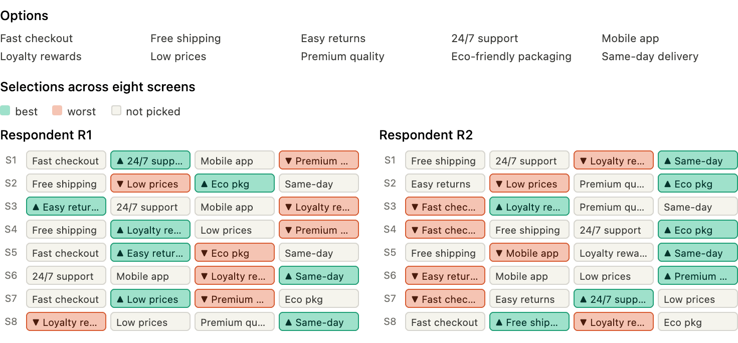
Users are repeatedly shown subsets of four options on a series of screens. We ask them to pick the best and worst out of those subsets. The raw results of a maxdiff question may look like this:

Now, we try to infer the a hidden preference order underlying these selections. The standard solution is to build probabilistic model of the selection process and then infer its parameters from the selections we made.

We assume that each respondent $i \in \{1,...,n\}$ has a hidden utility value $u_{i,k}$ for each option $k \in \{1,...,m\}$. The assumption is that given a subset of options $S$, items with higher scores are more likely to be selected as the top option, lower scores make a worst option selection more likely:

$$ p(\text{best}=b)=\frac{e^{u_{ib}}}{\sum_{k \in S} e^{u_{ik}}}, \quad p(\text{worst}=w)=\frac{e^{-u_{iw}}}{\sum_{k \in S} e^{-u_{ik}}} $$

Each respondent sees a series of screens $j \in \{1,…,l\}$, seeing the options $S_{i,j} \subset \{1,...,m\}$and making a selection for the best and worst items, $b_{i,j} \in S_{i,j}$ and $w_{i,j} \in S_{i,j}$, independently. This means that for a given utility vector and selection, we have:

$$ p(b_{:,:},w_{:,:}|S_{:,:}, u_{:,:})= \prod_{i,j} p(\text{best}=b_{i,j} | S_{i,j},u_{i,:}) \cdotp(\text{worst}=w_{i,j} | S_{i,j},u_{i,:}) $$

One could stop here with the model: It is easy to find a maximum a posteriori (MAP) estimate of the utilities $u_{{i,k}}$, or do a simple counting how many best and worst selections each items has by respondent and ordering the items accordingly as a proxy. However, this discards an important piece of information: The utilities of the items are likely correlated between the respondents.

Let us fix a respondent R1. Maybe, the choices of R1 by themselves do not give strong signal on whether they like options A or B better. However, if all the other respondents like B better than A, it is likely that so will R1. Or getting more advanced, maybe we know from other participants that respondents who like option C tend to also like option A. The result is that any signal on options C for R1 is highly informative about option A for R1. We do not want to loose these signals.

Therefore, we assume that the utility values $u_{i,k}$ are distributed according to a population distribution:

$$ u_{i,:} \sim \mathcal{N}(\mu,\Sigma) $$

Here, $\mu \in \mathbb{R}^m$ and $\Sigma \in \mathbb{R}^{m \times m}$ are the population-level parameters. This allows us to model population-wide trends, such as certain options tending to be more popular then others, or the popularity of options being correlated. The final part of the model is that we assume a prior belief on the population-level parameters, $\mu \sim p(\mu)$, $\Sigma \sim p(\Sigma)$. This is a broad, uninformative normal distribution for $\mu$ and LKJ-Cholesky (correlation) + Half-Normal (variance) for $\Sigma$.

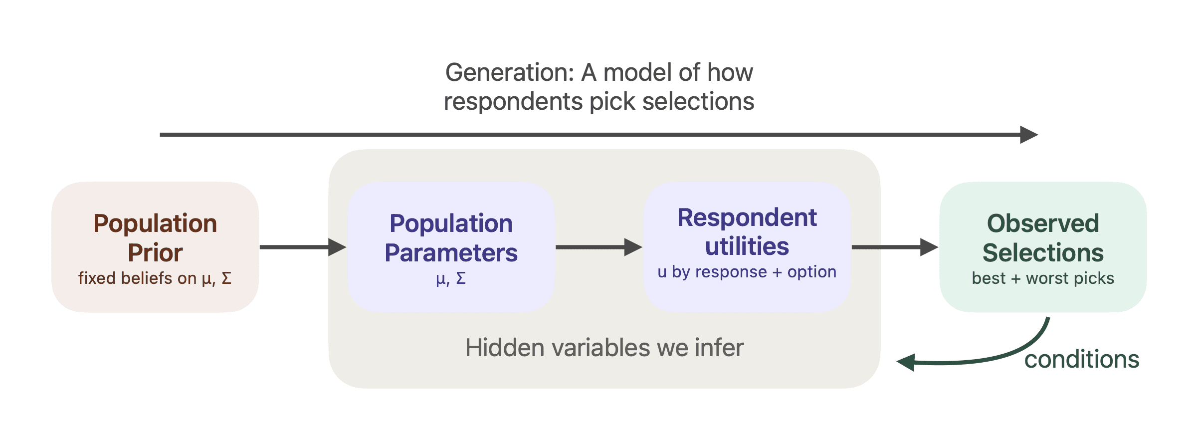
Let us look at this again from a high level: We built a model that describes how populations fill out maxdiff questions. The population mean and variance is sampled from an uninformative normal, then each respondents’ utilities for each option, $u_{{i,k}}$ is sampled from the population-level parameters $\mu$ and $\Sigma$, and finally, the best and worst selections on each screen are made based on their utilities. In other words, we can describe the joint probability $p(\mu,\Sigma,u_{:,:}b_{:,:},w_{:,:}$). How, does this help? We can only observe $b_{:,:},w_{:,:}$ (the best and worst items picked); $\mu,\Sigma,u_{:,:}$ (the population parameters and per-respondent utilities) are hidden. However, those hidden parameters are the ones we are most interested in for our analysis. We want to know how they behave conditionally on the selections we observed. In other words, we would like to sample from

$$ p(\mu,\Sigma,u_{:,:}|b_{:,:},w_{:,:}) $$

💡 We could also try to find the MAP estimate of the hidden parameters, but sampling gives us free uncertainty estimation on top!

If we could sample from the conditional distribution above, we could estimate the underlying population- and per-respondent utilities by taking the mean on a few samples. However, the direction of the sampling process is opposed to that: We first sample the population parameters, from that we sample the per-respondent utilities, and from the utilities, we sample the selections. A first naive conditional sampling algorithm could look like this:

This algorithms allows us to correctly infer the underlying population parameters! Unfortunately, the incidence rate on the conditional acceptance is tiny: We are basically simulating random populations and hope to find instances where the respondents happened to match our observation.

The solution is NUTS

Luckily, there is a more efficient algorithm: No-U-Turn Sampler (NUTS). The algorithm solves a more general problem: Suppose we have a probabilistic process with hidden variables $z$ and observable variables $x$. The models itself is defined through a joint probability distribution, $p(z,x)$. NUTS allows us to efficiently sample from $p(z|x)$, that is, the distribution of the hidden variables given the observed variables. The only input required is a closed form of the conditional log likelihood:

$$ \nabla_z \log p(z|x) $$

Luckily, log likelihood gradients of conditionals are often available in closed form, even if the log likelihood itself is infeasible. The reason for this is that normalization constant in Bayes theorem can be dropped through the differentiation: $p(z|x)=p(x|z) \cdot p(z)/p(x)=p(x,z)/p(x)$. Note that $p(x,z)$ is directly available in closed form in our model definition, but $p(x)$ is an integral over all possible $z$. Since $p(x)$ is independent from $z$, we can write:

$$ \nabla_z \log p(z|x) =\nabla_z (\log p(x,z) - \log p(x))=\nabla_z \log p(x,z) $$

This makes it possible to automatically sample from general hidden-variable models via auto-differentiation through libraries such as pymc or STAN.

So how does this apply to our problem? We have hidden variables $z=(\mu,\Sigma,u_{:,:})$ and observed variables $x=(b_{:,:},w_{:,:})$, as well as a closed-form expression for $p(\mu,\Sigma,u_{:,:},b_{:,:},w_{:,:})$. Through NUTS, we can sample from $p(\mu,\Sigma,u_{:,:}|b_{:,:},w_{:,:})$. Through the conditional samples of the hidden variables, we can estimate their underlying distributions. In practice, we are mostly interested in the expected population-level and individual utilities.

💡 Since rankings are relative between the options, we can only identify the utilities up to a constant. Therefore, in practice, we shift the utility samples to have zero-mean in the option dimension for each respondent: Instead of $u_{i,k}$, we use $u_{i,k}-\text{avg}_{k'}[u_{i,k'}]$

Putting the parts together

We construct a Hierarchical Bayes model that describes how a population responds to MaxDiff questions. The model’s hidden parameters encode the information we are most interested in: How much respondents like the options compared to each other. To estimate these parameters, we sample from the model conditioned on the observations we made. This allows us to estimate the hidden preference order with uncertainty quantification.